When and How to Snowflake Dimension Sources : SSAS Design Part 1
Reposted from Jason Thomas blog with the author's permission.
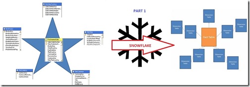
One of the best practices while designing a SSAS solution is to decouple your source database (which is in ideal cases, the data warehouse or the data mart but could also be an OLTP database) with the help of a semantic layer or view layer. Even though the Data Source View (DSV) of Analysis Services does provide a semantic layer, it is best to do all your intended operations/calculations within a SQL view and then use that view as the source of your dimensions and facts in the DSV. This will make sure that if the query for a dimension or fact needs to be changed at a later point of time, the SSAS solution need not be opened and make life easier for the DBA who is maintaining the system. It also has some performance benefits for the cube processing in the case of complex queries, which is beyond the scope of this post. This post tries to discuss a scenario in which you would want to snowflake your dimensions in the view layer (and not the scenarios in which you would want to snowflake your dimensions in the relational database or SSAS). Before all the Kimball enthusiasts come to bash me up, hear me out when I say that my preferred option would be to use the denormalized dimensions to create the popular star schemas. Even if the dimension is snowflaked in the relational database, I usually end up making a view on top of these normalized tables which will denormalize them into a single dimension giving a star schema look to the dimensions in the DSV. I am completely for the star schemas because of it’s simple, easy to understand and maintain structure. With this, I would also like to clear a popular misconception that the star schema is the best model for SSAS because of performance benefits due to lesser joins. Actually for large dimensions, the star schema would take longer time for cube processing than the snowflake schema and you can get a taste of this from a demo in MVP Ashwani Roy’s (blog | twitter) presentation on Analysis Services Best Practices.
Vincent Rainardi (blog) has written an excellent post on When to Snowflake your dimensions in the data warehouse side, which would be a good read prior to this post. If your data modeller generally follows a star schema approach and has already taken care of the concepts outlined in the above article by snowflaking appropriately, you would be lucky enough to just create the view layer as the exact copy of your data warehouse. Else have a look at the scenario below while making your view layer-
-
Multiple lower levels for the dimension (Scenario 1)
-
Multiple facts coming at multiple granularity (Scenario 2)
-
Multiple levels joining to the same parent (Scenario 3)
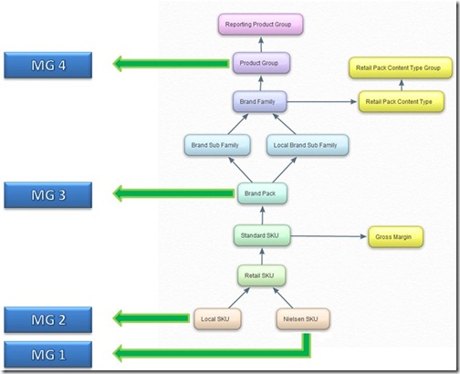
We will use the following Product dimension as an example for explaining the three scenarios.

Scenario 1 – Multiple Lower Levels
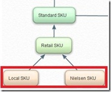
Consider the above figure where there are multiple lower levels (Nielsen SKU and Local SKU) in the dimension. Even though SSAS can handle multiple lower levels, it is always better to create a surrogate key which can be used as the dimension key (Read this post to learn how to create a dimension with multiple column key). For this scenario, the following views would be created in the view layer which would be then used as such in the DSV:-
a. View for dummy level – For the dummy level key, a surrogate id or sequence id can be used as it would be unique. The view would be of the following format SELECT // SID as dummy level key and the other two as foreign keys SID, LocalSKU_ID#FK, NielsenSKU_ID#FK FROM <table> // View for Local SKU and attributes SELECT Local_SKU, RSKU#FK FROM <table> // View for Nielsen SKU and attributes SELECT Nielsen_SKU, RSKU#FK FROM <table>
It is to be noted that the attributes / entities are taken only till the level of Retail SKU because Scenario 3 (multiple levels joining to the same parent) applies at Retail SKU level.
Now, why do we have to snowflake in this scenario? Let us see how the denormalized table would be for the same three levels
|
SID |
LSKU |
NSKU |
RSKU |
|
1 |
L1 |
NULL |
R1 |
|
2 |
L2 |
NULL |
R2 |
|
3 |
NULL |
N1 |
R1 |
|
4 |
NULL |
N2 |
R2 |
|
5 |
NULL |
N3 |
R2 |
Usually, I replace the NULLs by –1 in my design to avoid using the Unknown Member feature of SSAS. If this table is taken as the dimension source for SSAS and the appropriate relations are specified as SID—>LSKU—>RSKU and SID—>NSKU—>RSKU, there would be errors during dimension processing saying that there are multiple parents for the same child (for eg, –1 for NSKU would point to R1 and R2 values for Retail SKU). Snowflaking the source views as shown above would solve this problem. Please note that the SSAS Product dimension would still be a single one which would contain all the attributes from the snowflaked source views.
The other scenarios would be covered in the subsequent posts. Meanwhile it would be great to know how much you agree or disagree on these points.
 |
Jason has been working with Microsoft BI tools since he joined the IT industry in 2006. Since then he has worked across SSAS, SSRS and SSIS for a large number of clients. He is currently working for Mariner and is based out of Charlotte, NC. His personal blog can be found at http://road-blogs.blogspot.com |
Tags: design


