Gary Strange has been working with the Microsoft OLTP/OLAP stack for nearly two decades. He is currently architecting and developing BI solution for tier 1 investment banks at Dealogic.

---

Introduction

In this document I will demonstrate how using the TOPN function in a DAX query doesn’t necessarily do what you may expect. For the purpose of this document I will query the rather familiar Adventure Works Database.

The audience for this article is primarily SQL developers translating their skills to DAX.

How does top work in SQL Server.

The top clause in SQL has for a long time been used as a filter mechanism to reduce the number rows processed by the SQL Server Engine. Used at the correct time in a query, it can significantly reduce the processing of large datasets and increase performance.

Using the TOP clause in SQL Server I can dramatically reduce the number index/data page reads required to satisfy a given query. For instance if I read the DateKey column from the DimDate table the query plan will show that the whole index (PK_DimDate_DateKey) is scanned.

If I execute the following command

set statistics io on
select DateKey from DimDate order by DateKey desc

Message Output:

Table 'DimDate'. Scan count 1, logical reads 45, physical reads 0, read-ahead reads 0, lob logical reads 0, lob physical reads 0, lob read-ahead reads 0.

 

Query Plan Node:

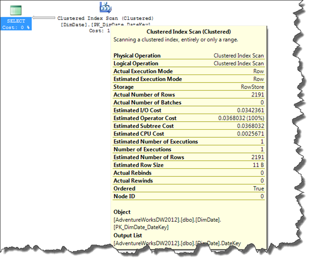
I can see that I get 2191 records from 45 page reads.

Now if I include the top clause…

set statistics io on
select top 10 DateKey from DimDate order by DateKey desc

Message Output:

Table 'DimDate'. Scan count 1, logical reads 2, physical reads 0, read-ahead reads 0, lob logical reads 0, lob physical reads 0, lob read-ahead reads 0.

Query Plan Node:

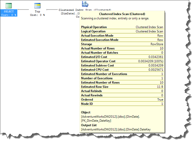
 I can see that I get 10 records from just 2 page reads, thus dramatically reducing the amount of work SQL Server had to do. This is only possible because a clustered index exists on this table and all the columns used in the query are available in the clustered index keys.

So we established how SQL Server behaves when using a top clause, now let’s take a look at what the SSAS Tabular server does.

How does top work in Tabular

DAX has a TOPN function, the function has a similar role to the SQL Server top clause but works in a slightly different way. This is due to the index strategy employed in the SQL Server query optimizer not being present in Tabular. SQL Server is able to seek to a node in an index and read a number of values, this is only achievable because the index values are listed in sorted order.

SSAS in tabular mode uses other optimization methods such as column based storage and value encoding to achieve high performance querying. Tabular always scans the whole column when using its TOPN function. We can see this happening by capturing the ‘DAX Query Plan’ event in the SQL Server Profiler.

If I execute the following command

evaluate values('Date'[Date])

I can capture the following physical query plan.

Spool_IterOnly<Spool>: IterPhyOp IterCols(0)('Date'[Date]) #Records=2191 #KeyCols=240 #ValueCols=0

     VertipaqResult: IterPhyOp #FieldCols=1 #ValueCols=0

 

You can see highlighted in yellow that 2191 column records were read. Now if I include the TOPN function and capture the plan I get the following…

evaluate topn(10, values('Date'[Date]), 'Date'[Date], 0)

 

PartitionIntoGroups: IterPhyOp IterCols(0)('Date'[Date]) #Groups=1 #Rows=10

   Spool_IterOnly<Spool>: IterPhyOp IterCols(0)('Date'[Date]) #Records=2191 #KeyCols=240 #ValueCols=0

     VertipaqResult: IterPhyOp #FieldCols=1 #ValueCols=0

'Date'[Date]: LookupPhyOp LookupCols(0)('Date'[Date]) DateTime

 

You can see highlighted in yellow that 2191 column records were read by the query engine. So on this occasion no optimizations were employed.

Now I can produce the same result set as the previous query, but this time using a table filter. Here is the query…

evaluate calculatetable( values('Date'[Date]), 'Date'[Date] >= DATEVALUE("7/22/2008"))

Spool_IterOnly<Spool>: IterPhyOp IterCols(1)('Date'[Date]) #Records=10 #KeyCols=240 #ValueCols=0

VertipaqResult: IterPhyOp #FieldCols=1 #ValueCols=0

This time you can see that the Vertipaq engine was able to constrain the number of column records it needed to read.

Now lets take a look at a more complex query. Below I have a query that simply aggregates all the Sales Amount values for each date in the date dimension.

evaluate
 addcolumns(
  summarize(
   'Internet Sales'
   , 'Date'[Date]
  )
 , "Sales", calculate(sum('Internet Sales'[Sales Amount]))
)

 

AddColumns: IterPhyOp IterCols(0, 1)('Date'[Date], ''[Sales])
   Spool_IterOnly<Spool>: IterPhyOp IterCols(0)('Date'[Date]) #Records=1124 #KeyCols=240 #ValueCols=0
     VertipaqResult: IterPhyOp #FieldCols=1 #ValueCols=0
   Spool: LookupPhyOp LookupCols(0)('Date'[Date]) Currency #Records=1124 #KeyCols=240 #ValueCols=1 DominantValue=BLANK
     VertipaqResult: IterPhyOp #FieldCols=1 #ValueCols=1

We can see again that 1124 column records have been read from the date dimension.

Now I can try out TOPN filtering or table filtering using CALCULATETABLE to see how they affect the plan.

First I’ll try TOPN…

evaluate
 addcolumns(
   topn(10,
    summarize(
       'Internet Sales'
       , 'Date'[Date]
     )
   , 'Date'[Date], 0)
   , "Sales", calculate(sum('Internet Sales'[Sales Amount]))
)

 

AddColumns: IterPhyOp IterCols(0, 1)('Date'[Date], ''[Sales])
  Spool_IterOnly<Spool>: IterPhyOp IterCols(0)('Date'[Date]) #Records=10 #KeyCols=1 #ValueCols=0
    PartitionIntoGroups: IterPhyOp IterCols(0)('Date'[Date]) #Groups=1 #Rows=10
       Spool_IterOnly<Spool>: IterPhyOp IterCols(0)('Date'[Date]) #Records=1124 #KeyCols=240 #ValueCols=0
         VertipaqResult: IterPhyOp #FieldCols=1 #ValueCols=0
        'Date'[Date]: LookupPhyOp LookupCols(0)('Date'[Date]) DateTime
       Spool: LookupPhyOp LookupCols(0)('Date'[Date]) Currency #Records=10 #KeyCols=240 #ValueCols=1 DominantValue=BLANK
        VertipaqResult: IterPhyOp #FieldCols=1 #ValueCols=1

 

As you can see, highlighted in yellow, 1124 column records are read by the Vertipaq engine. Now let’s get the same result but this time using a table filter…

evaluate
 calculatetable(
 addcolumns(
   summarize(
    'Internet Sales'
    , 'Date'[Date]
   )
   , "Sales", calculate(sum('Internet Sales'[Sales Amount]))
  )
 , 'Date'[Date] >= DATEVALUE("7/22/2008")
)

 

AddColumns: IterPhyOp IterCols(1, 2)('Date'[Date], ''[Sales])
  Spool_IterOnly<Spool>: IterPhyOp IterCols(1)('Date'[Date]) #Records=10 #KeyCols=240 #ValueCols=0
    VertipaqResult: IterPhyOp #FieldCols=1 #ValueCols=0
  Spool: LookupPhyOp LookupCols(1)('Date'[Date]) Currency #Records=10 #KeyCols=240 #ValueCols=1 DominantValue=BLANK
    VertipaqResult: IterPhyOp #FieldCols=1 #ValueCols=1

As you can see on this occasion only 10 column records were read by the Vertipaq engine. The engine was also able to produce a less complex query plan with fewer operators.

From these results we can see that the Vertipaq engine is unable to optimize top clauses in the same way SQL server does. On small data sets the impact in negligible but on larger datasets the performance impact maybe undesirable.

The Vertipaq engine does have a benefit to this unfiltered top implementation in that the result set is cached so consequent queries that use an alternative sort order do not need make new Vertipaq scans but can read data from cache.

Let’s start by looking at the execution steps created when I run the CALCULATETABLE style filter. On this occasion I will query the fact table as there is more data and this will help us identify activity on the Vertipaq engine.

If I execute the query below

evaluate
 addcolumns(
  calculatetable(
   summarize(
     'Sales'
     , 'Date'[DateDescription]
    )
   , 'Date'[DateDescription] <= "2007/01/10"
  )
 , "Sales", calculate(sum('Sales'[SalesAmount]))
)

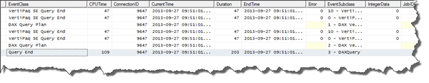
I get the following profile details…

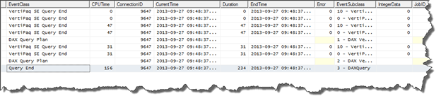
The first two calls represent the statistics gathering stage of the query execution. As the DAX query engine has a rule based optimizer it first asks questions about the size and shape of data involved in the query it needs to process. The next line in the output is the Logical plan. Described in a verbose manner the logical plan is the strategy the query engine will use to solve the query. The line(s) after that are the Vertipaq scans needed to gather data in order to complete the query. Data scanned in the initial statistics gathering stage is cached and can be reused later in the query execution stage. So you may find that a Vertipaq scan takes 0 seconds. This is because that scan was previously completed in the statistics gathering stage.

If I now execute a query that gets the last 10 values, the equivalent of a top descending.

evaluate
 addcolumns(
   calculatetable(
     summarize(
       'Sales'
        , 'Date'[DateDescription]
      )
    , 'Date'[DateDescription] >= "2009/12/21"
   )
  , "Sales", calculate(sum('Sales'[SalesAmount]))
)

I get the following profile details…

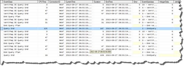
Again we see the same pattern. We can see that the second query* took half the time of the first query to execute. We can assume that it was able to make some use of the cache already created in the first query. You can see that both queries needed to make the same execution steps to solve the request.

* Entries below the blue row.

No let’s take a look at what is happening when we use TOPN.

I first ask for the top 10 descending.

evaluate
 addcolumns(
   topn(10,
     summarize(
      'Sales'
      , 'Date'[DateDescription]
     )
     , 'Date'[DateDescription], 1
    )
  , "Sales", calculate(sum('Sales'[SalesAmount]))
)

 I get the following profile details…

Then I ask for the top 10 ascending.

evaluate
addcolumns(
topn(10,
summarize(
'Sales'
, 'Date'[DateDescription]
)
, 'Date'[DateDescription], 0
)
, "Sales", calculate(sum('Sales'[SalesAmount]))
)

I get the following profile details…

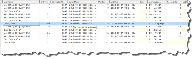
In the second query* I can see that the optimizer needed to make less scans to gather statistics and the one scan it did make it could read from cache as it has zero duration. We can see that the second query took a quarter of the time of the first query to execute. This is because it was able to make good use of the cache created in the first query.

* Entries below the blue row.

Conclusion

The TOPN function offers us some interesting behaviour to be considered when designing a DAX query. There are many articles in technical communities that condemn functions or behaviours, I think this whole mind set is wrong and this article is certainly not making a plea, for or against, the usage of TOPN. My hope is to simply enlighten and provoke thought when it comes to query design. Hopefully you will have also gained some insight into the mysterious DAX execution plan and are now a little more comfortable with dissecting it and performing you own exploratory experiments on the SSAS Tabular Server.