LastNonEmpty in Tabular mode : Part 1
Reposted from Jason Thomas blog with the author's permission.
My experience as a consultant has mostly been in the manufacturing sector and no wonder, I had frequent encounters with the notorious LastNonEmpty aggregation type in SSAS. I wouldn’t be exaggerating if I say that I had struggled quite a bit to understand and adapt this aggregation type to my needs when dealing with inventory, stock and status related data. I had dealt with varying scenarios but never thought of classifying these findings until a chance discussion with Javier Guillen (blog | twitter) prompted me otherwise. Together, we went through the scenarios and tried classifying them as well as applying them to the tabular mode and this post will be the first part of that effort.
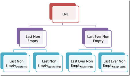
For the sake of simplicity, we adapted our discussions to the manufacturing scenario and the key dimensions used in the explanation below would be Time, Store and Product. However, this can be easily translated to other scenarios where the LastNonEmpty might be required. The LastNonEmpty (LNE) scenarios can be broadly classified into 2:- the typical Last Non Empty behavior of SSAS (where you would want to find the last non empty value within the selected time period) and the Last Ever Non Empty (credit for term usage - Chris Webb in this post) behavior (where you would want to find the last non empty value from all preceding time periods instead of just the selected time period). These types can be further broken down to at an overall level or at a store level as is shown in the chart below.
Let me briefly try to explain the four scenarios with an example.
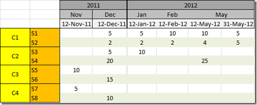
Assume that S1 - S8 are stores and C1, C2, C3, C4 are their parent groups as shown in the figure. The stock for each of the stores as well as the date in which they were recorded is also shown above. Now, the 4 LNE scenarios are given below:-
1) Last Non Empty(All Stores)
for C1 in 2012: 5+5 = 10 (last non empty date is 31-May-2012)
for C2 in 2012: 25 (last non empty date is 12-May-2012)
for C3 in 2012: None (no value in 2012)
for C4 in 2012: None (no value in 2012)
for Total in 2012: 5+5 = 10 (last non empty date is 31-May-2012)
This is equivalent to the LastNonEmpty aggregation type in SSAS multi-dimensional, where the last non empty date is calculated across all the stores within the selected time period and the values in that date are summed up.
2) Last Non Empty(Each Store)
for C1 in 2012: 5+5 = 10 (last non empty date is 31-May-2012 for both stores)
for C2 in 2012: 10+25 = 35 (last non empty date is 12-Jan-2012 for S3 and 12-May-2012 for S4)
for C3 in 2012: None (no value in 2012)
for C4 in 2012: None (no value in 2012)
for Total in 2012: 5+5+10+25 = 45 (sum of all the last non empty dates for each store)
Here, as shown in the example, the last non empty value is calculated for each store within the selected time period and then summed up. The equivalent of this aggregation type in SSAS multi-dimensional has already been explained by Teo Lachev in this post.
3) Last Ever Non Empty(All Stores)
for C1 in 2012: 5+5 = 10 (last non empty date is 31-May-2012)for C2 in 2012: 25 (last non empty date is 12-May-2012)
for C3 in 2012: 15 (no value in 2012, but there is value in 12-Dec-2011 for S6)
for C4 in 2012: 10 (no value in 2012, but there is value in 12-Dec-2011 for S8)
for Total in 2012: 5+5 = 10 (last non empty date is 31-May-2012)
Here, the last non empty date is calculated across all the stores from the very first date in the database to the last date of the selected time period and the values in that date only are summed up. Note that the last non empty date need not belong to the selected time period here, as is seen from the values for C3 and C4. The equivalent of this aggregation type in SSAS multi-dimensional has already been explained by Chris Webb in this post.
4) Last Ever Non Empty(Each Store)
for C1 in 2012: 5+5 = 10 (last non empty date is 31-May-2012)for C2 in 2012: 10+25 = 35 (last non empty date is 12-Jan-2012 for S3 and 12-May-2012 for S4)
for C3 in 2012: 10+15 = 25 (no value in 2012, but there is value in 12-Nov-2011 for S5 and 12-Dec-2011 for S6)
for C4 in 2012: 5+10 = 15 (no value in 2012, but there is value in 12-Nov-2011 for S7 and 12-Dec-2011 for S8)
for Total in 2012: 10+35+25+15 = 85 (sum of all the last non empty dates for each store)
Here, the last non empty date is calculated for each store from the very first date in the database to the last date of the selected time period and the values in that date are summed up for each store. Note that the last non empty date need not belong to the selected time period here, as is seen from the values for C3 and C4. It is not possible to have a really well performing method in SSAS multi-dimensional for this aggregation type without insanely extrapolating the fact data; this leaves us with only the extremely slow choice of making a calculated measure.
DAX is very powerful for performing such calculations and by the end of this series, you will see the performance gains that comes with having these scenarios in SSAS tabular. Let me go ahead and give the solutions for the first two types of Last Non Empty in DAX. I am using the Contoso database for my examples and they can be downloaded from this location.
1) Last Non Empty(All Stores)
An example of this scenario is when the product stock for all stores are recorded on a regular interval on the same date (daily, weekly, monthly, etc). As long as all the stores have data for the same dates, this formula will work in calculating the last non empty value. This is the simplest calculation of all the four and can be done using the DAX formula below
LNE_1:= Calculate (
Sum ( FactInventory[OnHandQuantity] ),
Filter ( DimDate, DimDate[DateKey] = Max ( FactInventory[DateKey] ) )
)
or
LNE_2:= Calculate (
Sum ( FactInventory[OnHandQuantity] ),
LastDate ( FactInventory[DateKey] )
)
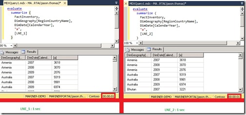
Performance wise, the results of both of them came back pretty fast and at almost the same time.
It is interesting to note that we are using FactInventory[DateKey] to get the last non empty date at which data is present. If we substitute the date key from the fact with the dimension in the above formula, we will get the DAX formula equivalent to the LastChild aggregation type in SSAS multidimensional.
LastChild:= Calculate (
Sum ( FactInventory[OnHandQuantity] ),
LastDate ( DimDate[DateKey] )
)
2) Last Non Empty(Each Store)
Now, this scenario is used when the stock is recorded for all stores on a regular interval but not necessarily on the same date for all the stores (However, it is assumed that the stock for all the products in a store would be taken on the same day). For eg, the stock for all the stores may be recorded monthly, but the stock would be recorded for some stores on the first week of the month, and some may be on the third or last week of the month. There are different ways in which you can write this calculation, and some of the ways I could find is written below:-
LNE_St_1:=
SumX (
Values ( DimStore[StoreKey] ),
Calculate (
Sum ( FactInventory[OnHandQuantity] ),
LastNonBlank (
FactInventory[Datekey],
1 )
)
)
or
LNE_St_2:=
SumX (
Values ( DimStore[StoreKey] ),
Calculate (
Sum ( FactInventory[OnHandQuantity] ),
LastDate ( FactInventory[Datekey] )
)
)
If you had read these posts (1 and 2), you might notice the recurring use of the pattern SumX(Values()) explained in those posts in both of the above formulas. You can also substitute the SumX(Values()) pattern with a SumX(Summarize()) pattern as shown below
LNE_St_3:=
SumX (
Summarize (
DimStore,
DimStore[StoreKey],
"LNE_P",
Calculate ( Max ( FactInventory[DateKey] ) )
),
Calculate (
Sum ( FactInventory[OnHandQuantity] ),
Filter (
All ( Dimdate ),
DimDate[DateKey] = [LNE_P]
)
)
)
The performance of all the formulas listed above were really good (all of them came back in 1 second). But the moment you add one more dimension to the formula (for eg, you need to find the last non empty for each store and product combination), there seems to be significant differences between the performance and I am currently doing some more testing on them (Well, might be a topic for another blog!). Meanwhile, you can go ahead and read the next part of this series in Javier’s blog.
Reference & Interesting Reads
1) Chris Webb - Last Ever Non Empty – a new, fast MDX approach
2) Teo Lachev - Last Non Empty Affairs
3) Jason Thomas - Changing Granularity of Leaf Level Calculations in SSAS Tabular
4) Javier Guillen - SCOPING at different granularities in DAX (Part I)
5) Paul te Braak - The Last Non-Empty Dilemma TABULAR Style
6) Hilmar Buchta - Sparse Snapshots in DAX / BISM Tabular
 |
Jason has been working with Microsoft BI tools since he joined the IT industry in 2006. Since then he has worked across SSAS, SSRS and SSIS for a large number of clients. He is currently working for Mariner and is based out of Charlotte, NC. His personal blog can be found at http://road-blogs.blogspot.com |


